

Doing More with More: Feature Transforms (Part 2)
Doing More with More: Feature Transforms (Part 2)
Building the World’s Greatest Recommender System Part 19


In this blog post, we continue answering the question of “What really goes into a machine learning model?” We will finish arming ourselves with the necessary input feature transforms.
Previously, we covered feature transforms which reduce the possible values for features, enabling us to represent them with a smaller range of values. However, in this post, we aim to do more, using more.
We will cover the popular transforms of one hot encoding dense features, hashing for sparse features, and embeddings for features, as well as n-gram transforms for combining features. These transforms, together, will help to complete the toolbox of feature transforms so that we have all the tools needed to develop features for a great recommender system at scale.
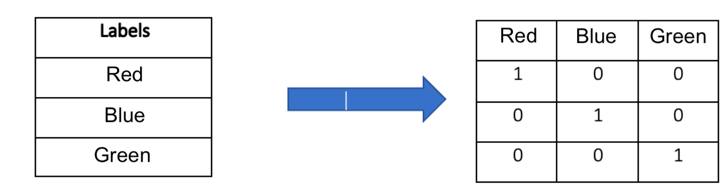
One-hot encoding is a technique to transform dense categorical variables into a format more usable by machine learning models. One hot encoding of dense features involves taking a feature with values that can be considered categorical, or non-numerical, and mapping it to a vector with as many elements as there are possible categorical values. That vector would have a single one, in the position corresponding to that categorical value, and zeros elsewhere. Say we have a user feature "favorite primary color" with three possible values: "red," "green," and "blue." One-hot encoding maps this feature into three binary vectors: "red" -> [1, 0, 0], "green" -> [0, 1, 0], "blue" -> [0, 0, 1]. As a result, categorical data takes on a numerical, vector format, which can be used by machine learning models, as they only take in and operate on numerical vectors. Additionally, the vector format, as opposed to a single numeric representation, such as "red" -> 1, "green" -> 2, "blue" -> 3, helps the model learn more quickly. It prevents the model from needing to discern, through training steps, that “red,” "green," and "blue" are independent categories and that “blue” (mapping to 3) is not greater than “red” (mapping to 1) in the same way that $3 is greater than $1.
Sparse features, unlike dense features, are features whose values could come from a huge possible list of values. For example, “last page that a user liked” could be a feature, and it could contain page “123456789” or “123456788” or “123456787.” Consequently, a one-hot representation of this feature would have high dimensionality with many zero values - if there are 1000000000 possible pages, then there would be a 1000000000 dimensional vector with one non-zero element.
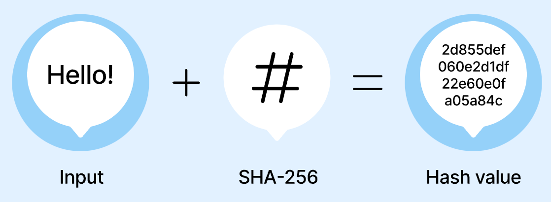
Hashing is an effective technique to reduce this dimensionality by mapping feature IDs to a fixed-size vector using a hash function. A simple hash-like function is the modulus, or remainder. In the case of the pages, we could do the remainder when divided by 1000, in which case there could now only be 1000 possible values, comprising a vector of 1000, and page “123456789” would map to a single 1 in the 789 position, page “123456788” would map to a single 1 in the 788 position, and page “123456787” would map to a single 1 in the 789 position. In practice, popular hash functions like SHA-256 or MD5 differ from this simple example in that they not guarantee that nearby values like “123456789” and “123456788” would have nearby hashed values, but aside from this, you can think of them as functioning like the remainder function. Thus, hashing sparse features can simplify storage and speed up computations by reducing the feature space.
A similar approach to reducing the dimensions of sparse features is generating embeddings, which are trainable smaller vector representations.
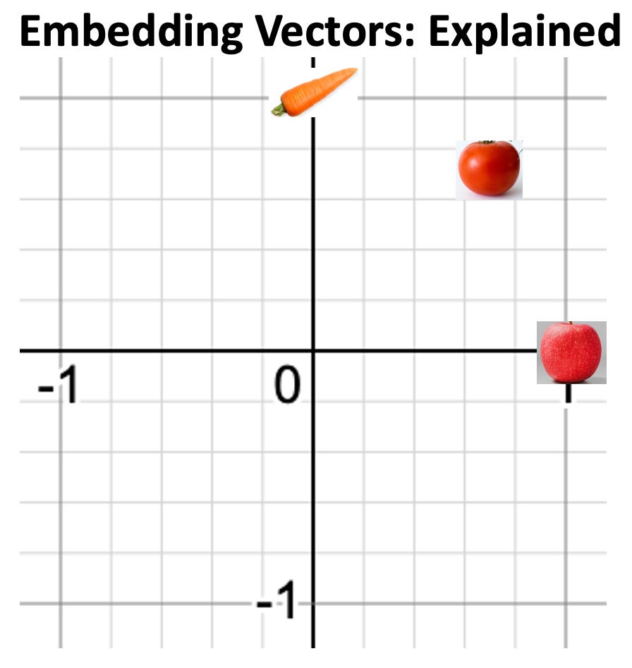
You may be familiar with the word “embedding” due to the hot new GPT (or other LLM). You can think of it as a vector of numbers that are intended to represent something. For example, if the first number in an embedding vector represented fruit and the second represented vegetable, a machine learning model could give embedding vector [1, 0] to an apple, [0, 1] to a carrot, and [0.5, 0.5] to a tomato (tomato actually would be [0.7071, 0.7071] normalized).
How do we get embeddings?
Given a user embedding vector and item embedding vector, we can train a model. We use a loss function which tells it “good model” when it predicts correctly and “bad model” when it predicts incorrectly, and then nudges the model through a technique known as gradient descent. We perform this training until user and item interaction predicted is the same as the true interaction between the items. For example, if the first number in a user’s embedding represents love of fruit and the second number represents love of vegetables and we had a user, Steve, who only ate fruit, the user embedding would be [1, 0]. We could use this information to train the embedding for an apple, if it was perhaps inaccurate, with the value [0.7071, 0.7071], representing equal fruit and vegetable qualities. To get a predicted value for Steve's interaction with apple, we would take a pairwise dot product between Steve’s embedding [1, 0] and the apple’s embedding [0.7071, 0.7071]. We compute a dot product by adding the product of each vector’s 1st element to the product of each vector’s 2nd element, getting 1*0.7071+0*0.7071=0.7071, suggesting we predict Steve is ok with apple. However, the true value of the interaction between fruit-lover Steve and the apple, would be 1. Consequently, we would rely upon gradient descent in model training to revise the embedding for apple to be [1, 0]. The dot product, now, would be 1*1+0*0 = 1, which is correct. Thus, with trainable vector representations for large, sparse vectors, we can reduce the dimensionality of sparse vectors significantly, and represent them in terms of characteristics (like fruit-ness and vegetable-ness). Through embedding representation of sparse input vectors from one component of a machine learning model, we can generate smaller, more meaningful vectors representing the traits of these otherwise meaningless sparse vectors, enabling a model to have access to more meaningful, useful feature values.
While features alone have value to a machine learning model, seeing features together can drive further value, a principle which n-gram transforms take advantage of. N-gram transforms generate combinations of features to capture relationships between adjacent items, enabling models to more easily find these relationships in training. For example, for user Amy, the feature “second last purchase price” may have value $19,999,999.99, and the feature “last purchase price” may have value $27.99 because Amy realized that she should significantly cut down on her spending moving forward after her 20 thousand dollar purchase. With “second last purchase price” and “last purchase price” combined in an n-gram with 2 features (a bigram), we would be able to capture behaviors of users like Amy. Consequently, the n-gram enables us to understand the context and relationships between features, giving us additional value. Perhaps an n-gram can make 1 + 1 = 3, if two features combined are more valuable than both features individually. In other words, perhaps “the whole is greater than the sum of its parts.”

Feature transforms are powerful tools in machine learning, enabling us to convert raw data into a more suitable format for machine learning models. By applying one-hot encoding, hashing and generating embeddings for sparse features, and performing n-gram transforms to combine features, we can enhance the quality of our data by projecting it into a more useful format based on sound human judgment. By enabling machine learning models to train and inference on this more useful format of data, we can continue to drive improvements in model performance.
If you benefited from this post, please share so it can help others.
Sources (All Content Can Be Found In Publicly Available Information; No Secrets):
https://arxiv.org/abs/2108.09373
https://unsplash.com/photos/silhouette-photo-of-man-on-cliff-during-sunset-_6HzPU9Hyfg (Zac Durant Image)
https://www.zencontrol.co.uk/the-whole-is-greater-than-the-sum-of-its-parts/ (Image)
https://infosecwriteups.com/breaking-down-md5-algorithm-92803c485d25 (Image)